Principal component analysis (PCA) is a statistical procedure that uses an orthogonal transformation to convert a set of observations of possibly correlated variables into a set of values of linearly uncorrelated variables called principal components. The number of principal components is less than or equal to the number of original variables. There are two methods in R to perform PCA. One is princomp, another is prcomp. I think these two methods are almost same.
#Use data iris as example
> myiris <- iris[,-5]
> pca1 <- princomp (myiris)
> pca2 <- prcomp (myiris)
> pca1
Call:
princomp(x = myiris)
Standard deviations:
Comp.1 Comp.2 Comp.3 Comp.4
2.0494032 0.4909714 0.2787259 0.1538707
4 variables and 150 observations.
> pca2
Standard deviations:
[1] 2.0562689 0.4926162 0.2796596 0.1543862
Rotation:
PC1 PC2 PC3 PC4
Sepal.Length 0.36138659 -0.65658877 0.58202985 0.3154872
Sepal.Width -0.08452251 -0.73016143 -0.59791083 -0.3197231
Petal.Length 0.85667061 0.17337266 -0.07623608 -0.4798390
Petal.Width 0.35828920 0.07548102 -0.54583143 0.7536574
#show the variables of pca result
> names (pca1)
[1] "sdev" "loadings" "center" "scale" "n.obs" "scores" "call"
> names (pca2)
[1] "sdev" "rotation" "center" "scale" "x"
> col <- rainbow(4, alpha=0.5)
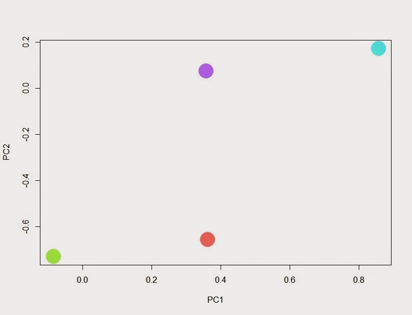
> plot (pca1$loadings, col=col, pch=16, cex=4) # plot PCA1 and PCA2
> plot (pca2$rotation, col=col, pch=16, cex=4) # plot PCA1 and PCA2
#show loadings value
> loadings(pca1)
Loadings:
Comp.1 Comp.2 Comp.3 Comp.4
Sepal.Length 0.361 -0.657 -0.582 0.315
Sepal.Width -0.730 0.598 -0.320
Petal.Length 0.857 0.173 -0.480
Petal.Width 0.358 0.546 0.754
Comp.1 Comp.2 Comp.3 Comp.4
SS loadings 1.00 1.00 1.00 1.00
Proportion Var 0.25 0.25 0.25 0.25
Cumulative Var 0.25 0.50 0.75 1.00
# show rotation value
> pca2$rotation
PC1 PC2 PC3 PC4
Sepal.Length 0.36138659 -0.65658877 0.58202985 0.3154872
Sepal.Width -0.08452251 -0.73016143 -0.59791083 -0.3197231
Petal.Length 0.85667061 0.17337266 -0.07623608 -0.4798390
Petal.Width 0.35828920 0.07548102 -0.54583143 0.7536574
#also show PCA1 and PCA2
> plot (pca1$loadings[1:4, 1],pca1$loadings[1:4,2], col=col, pch=16, cex=4)
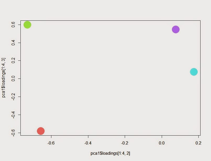
#plot PCA2 and PCA3
> plot (pca1$loadings[1:4, 2],pca1$loadings[1:4,3], col=col, pch=16, cex=4)
> plot (pca2$rotation[1:4, 2],pca2$rotation[1:4,3], col=col, pch=16, cex=4)
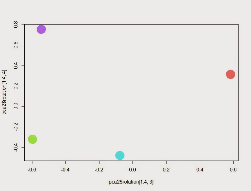
# plot PCA3 and PCA4
> plot (pca2$rotation[1:4, 3],pca2$rotation[1:4,4], col=col, pch=16, cex=4)
> plot (pca1$loadings[1:4, 3],pca1$loadings[1:4,4], col=col, pch=16, cex=4)
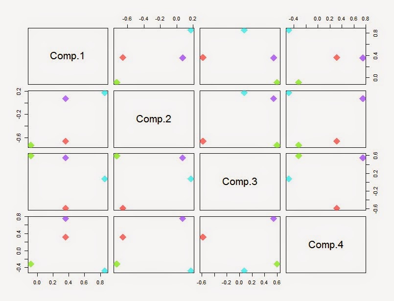
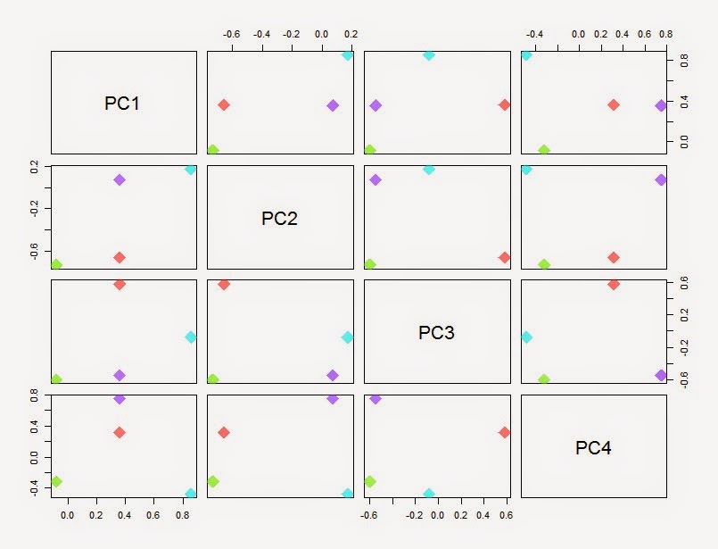
> pairs (pca1$loadings, col=col, pch=18, cex=3)
# plot all component
>
pairs (pca2$rotation, col=col, pch=18, cex=3)